6. vnl: Numerics

Chapter summary: C++ can be like Matlab, but faster and more powerful.

The numerics library, vnl is intended to provide an environment for numerical programming which combines the ease of use of packages like Mathematica and Matlab with the speed of C and the elegance of C++. It provides a C++ interface to the high-quality Fortran routines made available in the public domain by numerical analysis researchers.

This release includes classes for

• Matrices and vectors. The library is based on the old TargetJr/IUE classes, which provide the standard operations without excessive overhead.
• Specialized classes for matrices and vectors with particular properties. Class vnl_diagonal_matrix provides a fast and convenient diagonal matrix, while fixed-size matrices and vectors allow "fast-as-C" computations (see vnl_matrix_fixed<T,n,m> and example subclasses vnl_double_3x3 and vnl_double_3).
• Matrix decompositions. Classes vnl_svd<T>, vnl_symmetric_eigensystem<T> , vnl_generalized_eigensystem.
• Polynomials. Class vnl_real_polynomial stores the coefficients of a real polynomial, and provides methods of evaluation of the polynomial at any x, while class vnl_rpoly_roots provides a root finder.

  Class vnl_real_npolynomial also stores the coefficients of a real polynomial, but possibly in more than one unknown.

  Class vnl_poly is a templated class which allows to work with e.g. integer-coefficient (but just single-variable) polynomials.

• Optimization. Classes vnl_levenberg_marquardt, vnl_amoeba, vnl_lbfgs, vnl_conjugate_gradient allow optimization of user-supplied functions either with or without user-supplied derivatives.
• Standardized homes for commonly used functions and constants. Class vnl_math defines constants (pi, e, eps...) and simple functions (sqr, abs, rnd...). To quote the header "That's right, M_PI is nonstandard!" Class numeric_limits is from the ISO standard document, and provides a way to access basic limits of a type. E.g. numeric_limits<short>::max() returns the maximum value of a short.

Most routines are implemented as wrappers around the high-quality Fortran routines which have been developed by the numerical analysis community over the last forty years and placed in the public domain. The central repository for these programs is the "netlib" server http://www.netlib.org/. The National Institute of Standards and Technology (NIST) provides an excellent search interface to this repository in its Guide to Available Mathematical Software (GAMS) at http://gams.nist.gov, both as a decision tree and a text search.

For reasons of modularity (see "Layering" in the Introduction Chapter of this book) the numerics library is split up into vnl and vnl-algo. Matrix and polynomial representations are in vnl while anything requiring the "netlib" software is in vnl-algo. The Fortran routines themselves are implemented outside vxl, viz. in one of the v3p ("3rd party software") libraries.

Compliance with the ANSI standard C++ library

The ANSI standard includes classes for 1-dimensional vectors (valarray<T>) and complex numbers ( complex<T>). There is no standard for matrices. The current vnl classes are not implemented in terms of valarray, as there is a potential performance hit, but in the future they might be.

6.1 Example: Basic matrix and vector operations

This section provides a brief tutorial in using the main components of vnl. The main components which vnl supplies are the vector and matrix classes. The basic linear algebra operations on matrices and vectors are fully supported. Some very brief examples follow, but for the most part the usage of the vnl_vector and vnl_matrix classes is (we hope) obvious and intuitive.

Using these is easy, and is often modelled on Matlab. For example, this declares a 3x4 matrix of double:

#include <vnl/vnl_matrix.h>
int main()
{
  vnl_matrix<double> P(3,4);
  return 0;
}

Operators are overloaded as expected, so if we have another 3x4 matrix Q, we can add the two like this

vnl_matrix<double> R = P + Q;

The vnl_vector is equally straightforward. Here we make a 4-element vector of doubles, premultiply it by P, and print the result:

vnl_vector<double> X(4);
vcl_cerr << P*X;

Several more examples are shown in the figure below.

The vnl matrices are indexed from zero, as in C. This is always a difficult decision for C++ matrix libraries, as mathematical matrices use indices starting from 1--the top left element of A is generally written a_11. However, efficiently achieving this in C or C++ is a little bit tricky, and can confuse some tools like Purify. In the end, it was decided that zero-based indexing was closer to being "not weird".

  vnl_matrix<double> A(3,3); // 3x3 matrix, elements not initialized
  vnl_matrix<double> B(3,3, 1.0); // 3x3 matrix, filled with ones.
  vnl_matrix<double> R(3,4); // Rectangular matrix
  vcl_cerr << "A is " << A.rows() << 'x' << A.columns() << vcl_endl
           << "A has a total of " << A.size() << " elements" << vcl_endl;
  A(0,0) = 2.0; // Set top-left component of A.
  A(3,3) = 0.0; // *** Error, (3,3) is outside the range of A.
  A.set_size(3,4); // Change size of A, invalidating elements.
  R.update(A, 0, 1); // Copy A into R, starting at (0,1): last 3 cols
  R.set_column(0, B.get_column(0)); // Copy 1st col of B into R
  vcl_cerr << R.extract(3,3, 0,1) // Print last 3 cols
           << R.get_n_columns(1, 3) const; // Ditto

  A.fill(0.0); // Set all elements of A to 0.0
  A.fill_diagonal(1.0); // Set diagonal elements to 1.0
  A.set_identity(); // Set A to identity matrix
  R = R.transpose(); // Make transposed copy, assign to R
  R.inplace_transpose(); // Transpose R without copying.
  A.flipud(); // Reverse order of rows of A
  A.fliplr(); // Reverse columns
  A.normalize_rows();  // Divide each row by its 2-norm
  A.scale_row(0, 2.0); // Multiply row 0 by 2
  vcl_memset(A.data_block(), 0); // Access A's raw storage
  fill(A.begin(), A.end(), 0.0); // Fill using STL iterators

  vnl_matrix<double> C = B + 0.1 * A; // Arithmetic
  C += 2.3;
  vnl_matrix<double> Csqrt = C.apply(sqrt); // Square root all elements
  element_product(Csqrt, Csqrt); // Should be equal to C, modulo roundoff

  vcl_cerr << A.fro_norm() // Print sum of squares of elements
           << A.min_value(); // Print minimum element

  if (A.is_zero(1e-8))
    vcl_cerr << "Each element of A is within 1e-8 of zero\n";
  if (A.is_identity(1e-8)) vcl_cerr << "(A - I) is_zero to 1e-8\n";

  A.read_ascii(vcl_cin); // Read A from standard input

6.1.1 Efficiency: Fixed-size matrices and vectors.

A C programmer looking at the above examples will immediately grumble about the inefficient memory allocation that is being performed. Let's look into the construction of P in more detail. One can guess that the line

vnl_matrix<double> P(3,4);

might result in a sequence of actions something like the following:

struct vnl_matrix<double> P;
P.rows = 3;
P.columns = 4;
P.data = new double[P.rows * P.columns];

The expensive part of this operation is the call to new, which might involve many instructions, and even a bit of operating system activity. (Typically a call to new or malloc will cost about as much as a 2x2 matrix multiply).

If the matrices are small, as in these examples, this cost is significant--if they're bigger than about 20x20 it is not so important. Always remember, when thinking about efficiency, to consider what else is going on in the program. For example, if a matrix is being read from disk, the time taken to read the matrix will be many times greater than a few copies. If you are about to do a matrix multiply (an O(n^3) operation after all), an O(n^2) copy or an O(1) new are not going to be hugely significant.

However, for small matrices we should try to avoid calls to new, and vnl provides some fixed-size matrices and vectors which do so. The templates which define these are called vnl_vector_fixed and vnl_matrix_fixed, and the template instances include the size of the vector or matrix in their parameters. A vector of double with fixed length 4 is defined using

    vnl_vector_fixed<double, 4>

with analogous syntax for matrices. Thus a more efficient version of the above sequence would be

#include <vnl/vnl_matrix_fixed.h>
#include <vnl/vnl_vector_fixed.h>
int main()
{
  vnl_matrix_fixed<double,3,4> P;
  vnl_vector_fixed<double,4> X;
  vcl_cerr << P*X;
  return 0;
}

It's a bit clumsy typing these long names, so it is common to use typedef to make shorter ones. Indeed, a few are supplied with vnl, for example vnl_double_3x4 (defined, of course, in a header called vnl_double_3x4.h). So a more compact rendition of our example is

#include <vnl/vnl_double_3x4.h>
#include <vnl/vnl_double_4.h>
int main()
{
  vnl_double_3x4 P;
  vnl_double_4 X;
  vcl_cerr << P*X;
  return 0;
}

Note again that in this example there will be no noticeable speedup, because 99% of the runtime will be spent on the last line, printing the vector.

Because some operations such as multiplication have been specially coded for the fixed-size classes, they are also made more efficient by knowing the sizes in advance. For example, this snippet

vnl_double_3x3 R;              // Declare a 3x3 matrix
vnl_double_3 x(1.0,2.0,3.0);   // Declare a 3-vector using
                               // local storage
vnl_double_3 rx = R * x;       // Multiply R by x and place
                               // the result in rx

is expanded by many compilers into an open-coded sequence of 9 multiplies and 6 adds.

6.1.2 Caveats when using the fixed-size classes

The fixed-size classes are optimally space efficient; sizeof(vnl_vector_fixed<double,4>) and sizeof(double[4]) are the same. To achieve this, it is necessary to decouple vnl_vector from vnl_vector_fixed, in the sense that neither inherits from the other. This means that you cannot pass a vnl_vector_fixed to a function that expects a vnl_vector without some conversion. Luckily, there is a cheap conversion operator from vnl_vector_fixed to vnl_vector_ref, which is a derived class of vnl_vector. This conversion operator will be applied behind the scenes in most cases, so you often don't have to worry about it.

double norm( vnl_vector<double> const& v );
...
vnl_vector_fixed<double,6> fixed_v;
double n = norm(fixed_v); // this will create a temporary
                          // vnl_vector_ref<double> const
                          // to pass to norm

The cost of the conversion is on the order of 1 pointer copy (data pointer) and 1 integer copy (length) for a vector and 1 pointer and 2 integers for a matrix.

Unfortunately, this is not the end of the story. According to the 1998 ISO C++ standard, user defined conversion operators will not be applied when determining candidate template functions. Therefore, the following snippet fails to compile.

template<typename T>
T norm( vnl_vector<T> const& v );
...
vnl_vector_fixed<double,6> fixed_v;
// no match for
//    norm(vnl_vector_fixed<double,6>)
// User defined conversion operators are not
// tried since norm is a template.
double n = norm(fixed_v);

For these cases, and other cases where the implicit conversion operator cannot be applied, you have to do the conversion explicitly using as_ref().

template<typename T>
T norm( vnl_vector<T> const& v );
...
vnl_vector_fixed<double,6> fixed_v;
double n = norm(fixed_v.as_ref()); // calls norm with
                                   // a vnl_vector_ref<double> const

When writing general purpose templated functions that are equally useful for both the dynamically allocated vnl_vector and statically allocated vnl_vector_fixed, it is often useful to provide a simple forwarding wrapper so that the user is spared the inconvenience of doing the explicit conversion.

template<typename T>
T norm( vnl_vector<T> const& v );  // real function
template<typename T, unsigned n>
inline
T norm( vnl_vector_fixed<T,n> const& v ) { // thin wrapper
  return norm( v.as_ref() );
}
...
vnl_vector_fixed<double,6> fixed_v;
double n = norm(fixed_v); // this calls the second norm

The final wrinkle with mixing vnl_vector and vnl_vector_fixed is that the conversion operators, both the implicit and explicit, create temporary vnl_vector_ref objects, which, according to the standard, cannot bind to non-const references. Therefore, you cannot pass these to a mutator function that modifies the values in your vector.

void mutator( vnl_vector<double>& v );
...
vnl_vector_fixed<double,6> fixed_v;
mutator(fixed_v); // the temporary object created by the
                  // conversion is const => cannot be
                  // passed to mutator.

The only solution to this is to explicitly force the temporary object to "give away" its const-ness, using the non_const() method in vnl_vector_ref.

void mutator( vnl_vector<double>& v );
...
vnl_vector_fixed<double,6> fixed_v;
mutator(fixed_v.as_ref().non_const());

The discussion above applies equally well to vnl_matrix and vnl_matrix_fixed.

6.2 Example: Matrix decomposition

The most frequently asked question about vnl_matrix is "where is the inverse method", and the answer is that the inverse is not defined as a method, because there are too many ways of forming it, each with different tradeoffs. If you really don't care to hear about these things, you can use the vnl_matrix_inverse class to compute an inverse object:

#include <vnl/algo/vnl_matrix_inverse.h>
int main()
{
  vcl_cerr << vnl_matrix_inverse<double>(A) * B;
  return 0;
}

If you want more control over how the inverse is taken, then you might want to look at vnl_inverse or at one of the decomposition classes.

TODO - order in general-specific, give flop counts, show decomps.

The following fragment demonstrates use of the vnl_svd<double> class to find the approximation of a 3x3 matrix F by the nearest matrix of rank 2

vnl_double_3x3 rank2_approximate(vnl_double_3x3 const& F)
{
  // Compute singular value decomposition of F
  vnl_svd<double> svd (F);
  // Set smallest singular value to 0
  svd.W(2,2) = 0;
  // Recompose vnl_svd<double> into UWV^T
  return vnl_double_3x3(svd.recompose());
}

A more extensive example of the use of linear algebra is provided in Figure 2, which contains a program to fit a hyperplane to points read from standard input.

#include <vnl/vnl_matrix.h>
#include <vnl/vnl_vector.h>
#include <vnl/algo/vnl_svd.h>
#include <vnl/algo/vnl_symmetric_eigensystem.h>
#include <vcl_iostream.h>

int main()
{
  // Read points from stdin
  vnl_matrix<double> pts;
  vcl_cin >> pts;

  // Build design matrix D
  int npts = pts.rows();
  int dim = pts.columns();
  vnl_matrix<double> D(npts, dim+1);
  for (int i = 0; i < npts; ++i)
  {
    for (int j = 0; j < dim; ++j)
      D(i,j) = pts(i,j);
    D(i,dim) = 1;
  }

  // 1. Compute using vnl_svd<double>
  {
    vnl_svd<double> svd(D);
    vnl_vector<double> a = svd.nullvector();
    vcl_cout << "vnl_svd<double> residual = " << (D * a).magnitude() << vcl_endl;
  }

  // 2. Compute using eigensystem of D'*D
  {
    vnl_symmetric_eigensystem<double>  eig(D.transpose() * D);
    vnl_vector<double> a = eig.get_eigenvector(0);
    vcl_cout << "Eig residual = " << (D * a).magnitude() << vcl_endl;
  }
  return 0;
}

6.2.1 Sparse linear solver

It is often the case that large linear systems have a sparse coefficient matrix, where many of the elements are zero. An algorithm for solving such systems is vnl_sparse_lu based on the c library, Sparse 1.3a, by Kenneth S. Kundert and Alberto Sangiovanni-Vincentelli. The algorithm solves the linear problem

Ax = b

by chosing a set of pivots for the matrix, A, and factoring it into lower and upper triangular form, i.e., LU decomposition. The solution, x, for a given b, is found by forward and back substitution. The class vnl_sparse_lu maintains the factored matrix so that solutions for any number of b (right hand side) vectors can be found without repeating the pivoting and factorization process. The factored matrix is also used to compute |A| as well as the solution of A^t x = b. An example of solving a linear system using vnl_sparse_lu:

#include <vnl/vnl_vector.h>
#include <vnl/vnl_sparse_matrix.h>
#include <vnl/algo/vnl_sparse_lu.h>
vnl_sparse_matrix<double> S(6,6);
S(0,0)=0.49; S(0,1)=-0.5;
S(1,0)=-0.5; S(1,1)=0.99; S(1,2)=-0.5;
S(2,1)=-0.5; S(2,2)= 0.99;
S(3,3)=0.99; S(3,4)=-0.5;
S(4,3)=-0.5; S(4,4)=0.99; S(4,5)=-0.5;
S(5,4)=-0.5; S(5,5)=0.99;
vnl_vector<double> b(6,0), x(6);
b[2]=0.5; b[3]=0.5
vnl_sparse_lu linear_solver(S, vnl_sparse_lu::estimate_condition);
linear_solver.solve(b,&x);
double det = linear_solver.determinant();
double rcond = linear_solver.rcond();
double upbnd = linear_solver.max_error_bound();
//
//Results
//
// x = { 1.1338, 1.11112, 1.06622, 1.06622, 1.11112, 1.1338 }
// det = 0.0121548
// rcond = 0.0375578 (reciprocal of the condition number)
// upbnd =  5.92331e-015 (upper bound on solution error)
//

Note that the algorithm does not require that A is a symmetric matrix. The operation code, estimate_condition, specifies that extra computation is carried out so that the condition number of the matrix and expected error can be determined. If these quantities are not needed then use the operation codes quiet or verbose.

6.3 Polynomials

The vnl_rpoly_roots class in vnl/algo is used to compute the roots (or "zeros") of a real polynomial. For example, given the cubic equation

     4 x^3 + 3 x^2 - 7 x + 5 = 0

we can compute the values of x using vnl_rpoly_roots. The first step is to collect the coefficients into a vector, listing from the highest power down. In the above example, we should make the vector

     [4, 3, -7, 5]

In C++, this could be written

     vnl_double_4 poly;
     poly[0] = 4;
     poly[1] = 3;
     poly[2] = -7;
     poly[3] = 5;

Having prepared the polynomial, we compute the roots:

     vnl_rpoly_roots roots(poly);

Now, roots contains the roots, which can be made use of, or simply admired. To facilitate the latter, we shall print them to the console:

     for (int k = 0; k < 3; ++k) // Cubic polynomial ==> 3 roots
       vcl_cerr << roots[k] << vcl_endl;

To get just the real or imaginary parts of the (generally complex) roots, convenience methods real(int) and imag(int) are provided. So to print only the real roots, one might use

     for (int k = 0; k < 3; ++k)
       if (roots.imag(k) < 1e-8)
         vcl_cerr << roots.real(k) << vcl_endl;

6.3.1 Implementation

The implementation is a wrapper for the fortran code in algorithm 493 from the ACM Transactions on Mathematical Software. This is the Jenkins-Traub algorithm, described by Numerical Recipes under "Other sure-fire techniques" as "practically a standard in black-box polynomial rootfinders". (See M.A. Jenkins, ACM TOMS 1 (1975) pp. 178-189.).

The algorithm fails if poly[0] is zero, so it's often good to try to write your problem so that the leading coefficient (i.e. poly[0]) is equal to 1.

6.4 Nonlinear Optimization

It is not uncommon in computer vision research to meet problems for which there is no known closed-form solution, and a common class of such problems are of the form "find , and , such that the function takes its minimum value". For example, fitting a line to a set of 2D points {(x_i,y_i) | i=1..n}. The problem is then to find a,b,c to minimize the sum of distances of each point to the line ( )

                  n   (a * x[i] + b * y[i] + c)^2
      f(a,b,c) = sum  ---------------------------
                 i=1         (a^2 + b^2)

In the case of line fitting, a closed-form solution can be found, but in many other problems, no such solution is known, and an iterative method must be employed.

In those cases, one needs a good, general purpose nonlinear optimization routine. Of course, such a panacea does not exist, so vnl provides several from which to choose. The factor that decides which is best is most frequently the amount of knowledge that one has about the form of the function. The more you know, the more quickly you can expect the optimization to proceed. For example, if you can compute the function's derivatives, you would expect to achieve better performance.

6.4.1 Choosing a minimizer

The routines provided in vnl may be arranged roughly in decreasing order of generality--and correspondingly, increasing order of speed--as follows:

1. vnl_amoeba: Nelder-Meade downhill simplex. The method of choice if you know absolutely nothing about your function, but fear the worst. It you think the function might be noisy (i.e. the error surface has many small pockets), or you don't trust it to have reasonable derivatives, downhill simplex is a good choice. If you want the code to run fast, it's not.
2. vnl_powell: Powell's direction-set method. Powell's method, like simplex, doesn't require that you supply the derivatives of with respect to , , and , but it does assume they are moderately well behaved.
3. vnl_conjugate_gradient: Fletcher-Reeves form of the conjugate gradient algorithm.
4. vnl_lbfgs: Limited memory Broyden Fletcher Goldfarb Shannon minimisation. Requires 1st derivatives. Considered to be the best general optimisation algorithm for functions which are well behaved (i.e. locally smooth without too many local minima.)
5. vnl_lbfgsb: Limited memory BFGS bounded minimisation. Requires 1st derivatives. Allows simple box inequality constraints.
6. vnl_levenberg_marquardt: The Levenberg-Marquardt algorithm for least-squares problems. This is usually the best method for any function which can be expressed as f(x) = (f_1 (x))^2 + (f_2(x))^2 + (f_3(x))^2 + \dots

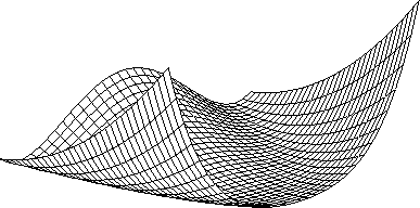
As an example of the use of the optimization routines, we'll use a common test case, the "notorious" Rosenbrock function:

     f(x, y) = (10*(y - x^2))^2 + (1-x)^2

The graph of is plotted in Figure 2.

6.4.2 Function objects, derived from vnl_cost_function

Running an optimization is a two step process. The first is to describe the function to the program, and the second is to pass that description to one of the minimizers. Functions are described by function objects, or "functors", which are classes which provide a method f(...) which takes a vector of parameters as input, and returns the error. Such functors are derived from vnl_cost_function:

     struct my_rosenbrock_functor : public vnl_cost_function { ... };

The function is a method in the derived class. Here's the continuation of the declaration of my_rosenbrock_functor.

       double f(vnl_vector<double> const& params)
       {
         double x = params[0];
         double y = params[1];
         return vnl_math_sqr(10*(y-x*x)) + vnl_math_sqr(1-x);
       }

Because a vnl_cost_function can deal with cost functions of any dimension, not just the 2D example here, my_rosenbrock_functor must tell the base class the size of the space it's working in. This is done in the constructor as follows:

       my_rosenbrock_functor():
         vnl_cost_function(2) {}

And we can now close the declaration of my_rosenbrock_functor:

     }

6.4.3 Running the minimization

In order to perform the minimization, a vnl_amoeba compute object is constructed, passing the vnl_cost_function.

my_rosenbrock_functor f;
vnl_amoeba minimizer(f);

Having provided an initial estimate of the solution in vector x, the minimization is performed:

minimizer.minimize(x);

after which the vector x contains the minimizing parameters.

6.4.4 Least-squares problems: The Levenberg-Marquardt algorithm.

The Levenberg-Marquardt algorithm provides only for nonlinear least squares, rather than general function minimization. This means that the function to be minimized must be the norm of a multivariate function. However, this often the case in vision problems, and allows us to use the powerful Levenberg-Marquardt algorithm. The Rosenbrock function can also be written as a 2D-2D least squares problem as follows:

f(x, y) = [ 10(y - x^2) ]
          [    1-x      ]

In this case, we need to make a class derived from vnl_least_squares_function. TODO

6.5 Design issues (Developer Topic)

This section documents some design decisions with which people might disagree. Please let me know how you feel on these issues. It's also a malleable to-do list. The most important consideration has been to provide simple lightweight interfaces that nevertheless allow for maximum efficiency and flexibility.

6.5.1 Computation in constructors

As noted above, a common model in this package is that the compute objects perform computation within the constructors. While this is slightly distasteful from a traditional C++ viewpoint, it offers a number of advantages in both efficiency and ease of use.

The philosophical argument, say in the case of SVD, is that SVD is a noun. The natural description is "The SVD of a matrix M" which is expressed in C++ as vnl_svd<double> svd(M) .

Storage for the results of a computation is provided by the compute object which is convenient, allowing client code to access only those results in which it is interested. Local storage is also more efficient, as objects are constructed at the correct size, and initialized immediately. In contrast, passing empty objects to a function will generally involve a resize operation, while returning a structure will incur a speed penalty due to the necessary copy operations.

Namespace clutter is avoided in the vnl_matrix class. While svd() is a perfectly reasonable method for a matrix, there are many other decompositions that might be of interest, and adding them all would make for a very large matrix class, even though many methods might not be of general interest.

The model extends readily to -ary operations such as generalized eigensystems, which combine two objects to produce others. Such operations cannot be methods on just one matrix.

6.5.2 Fixed-size classes

The classes which provide for fast fixed-size matrices and vectors are essential in a system which wants to make claims for efficiency. In addition, a great many uses of these objects do know the size in advance. In this case code using say vnl_double_3 is more efficient (as well as more self-documenting) than the equivalent referring to a vnl_vector of unknown size.

6.5.3 Transposing for Fortran

In calling Fortran code, the first difficulty that becomes apparent is that Fortran arrays are stored column-wise, while traditional `C' arrays are stored row-wise - a trend that is followed by the vnl_matrix class. One solution is simply to store C++ arrays column-wise, and this was an early plan for the IUE.

I have not done anything to alleviate this for two reasons - most routines we call are expensive enough (i.e. ) that the copy operation is only a small performance hit. Secondly, many decompositions satisfy a transpose-equivalence relationship. For example suppose we wish to use a Fortran matrix multiply which has been hand-optimized for some particular machine. Such a routine may be declared

mmul(A, B, C) // Computes C = A B, fortran storage

To use this with row-stored arrays, we recall the simple identity

C = (C')' = (B' A')' = AB

and therefore call mmul(B, A, C), reversing the order of parameters and . The fortran code will lay down the result of into the columns of , thereby computing from the point of view of the caller.

This however, doesn't apply to the vnl_svd<double>, as algorithms generally require only the "economy-size" version where size(U) = size(M) in . This is flops rather than for the full size one. Using the transpose-equivalence would mean a doubling of the computation time, as the "economy-size" decomposition is only implemented for . If someone does need the full size decomposition, a flag could be added or a new vnl_svd class written.

6.6 Future work

Many of the existing methods are unimplemented, or could benefit from optimization. Users can contribute code to address these deficiencies based on the existing examples, and using the conversion hints in Appendix~A. In addition there are many algorithms that ought to be included, listed roughly in order of priority:

• Additional matrix decompositions in the same vein, including an updateable QR, a basic LU, etc.
• Choice of back-end functions--for optimization one might prefer Powell, or even simulated annealing. For matrix decompositions, particular users might prefer to interface to NAG or IMSL routines. These choices must be allowed to be made easily, thereby encouraging the comparison of algorithms and of alternative implementations.
• Many classes are defined as double-only rather than templated. I will use default template arguments when the compilers support them.

This document was generated on May, 1 2013 using texi2html 1.76.